Data comes in a variety of shapes and forms. A dataset can be as simple as a table containing data in the form of rows and columns, and as complex as images and videos with multiple colour channels.
In the context of machine learning, different types of algorithms are developed that target a specific set of problems using data in a particular format. These algorithms expect input data to be in specific format.
In this article, you will see how to convert data into the right input shape before you can use it to train different types of deep learning algorithms in Python’s TensorFlow Keras library.
You will be working with the three main data formats that you will mostly encounter while training your deep learning algorithms in TensorFlow Keras.
- Tabular Data
- Image Data
- Sequence/Time Series Data
Tabular Data
Tabular data, also known as structured data, is data stored in the form of tables. The table columns correspond to data attributes whereas table rows correspond to data instances.
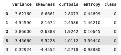
The following screenshot shows an example of tabular data that consists of various features of a bank note image. The class column contains information on whether or not a bank note is fake.

Salient Features of Tabular Data
- In tabular data the data instances are independent and have no relationship with each other.
- Tabular data is highly structured and easiest to manage for machine learning algorithms
- Among deep neural networks, densely connected neural networks (DNN) are mostly recommended for training with tabular data. However, results show that with sufficient amounts of data, classific machine learning algorithms such as random forest and the xgboost algorithm return performances comparable to a DNN.
As discussed, a densely connected neural network is most suitable for solving problems involving tabular data as the input.
Let’s understand how to specify input shape for tabular data while training DNN implemented in the Tensorflow keras.
As a sample problem, you will be training a DNN classifier which detects fake bank notes given bank note image features such as variance, skewness, curtosis, and entropy. The dataset is freely available at this Kaggle link:
https://www.kaggle.com/ritesaluja/bank-note-authentication-uci-data
Now let’s do a bit of Python coding.
If you are familiar with Python and deep learning, the upcoming section is going to be straightforward with some calls to Python’s TensorFlow Keras library functions.
If you are not familiar with Python or deep learning, just focus on the input data shape parameter in an upcoming code snippet because this is what this article mainly explains.
The following script imports the required Python libraries:
import numpy as np

import pandas as pd
The script below reads the CSV file containing our tabular data into a Pandas dataframe which is a data structure for storing tabular data. In the output, you can see the first five rows of the dataset.
dataset = pd.read_csv("/content/BankNote_Authentication.csv")

dataset.head()
Output:
The following script prints the shape of the dataset.
dataset.shape
Output:
(1372, 5)
The above output shows that our dataset consists of 1372 rows and 5 columns. The first dimension in the shape tuple refers to the sample, or instance dimensions and is normally not used when specifying the input shape for TensorFlow Keras models.
Next, you will train a DNN using the variance, skewness, curtosis, and entropy attributes from the dataset, to predict whether a bank note is fake or not (value in the class column.
To do so, you need to divide your dataset into the features and labels. The feature set X, as shown in the script below consists of all the columns except “class” whereas the corresponding label set will consist of values from the “class” column./
X = dataset.drop(["class"], axis = 1)

y = dataset.filter(["class"], axis = 1)
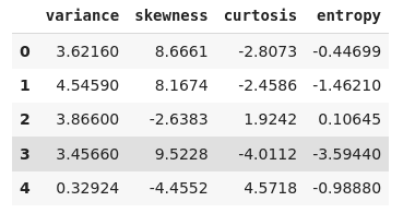
Let’s display our feature and label sets.
X.head()
Output:
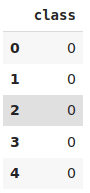
y.head()
Output:
The next step is to divide the dataset into training and test sets. The training set is used to train a deep learning algorithm whereas the test set is used to evaluate the performance of the trained model on unseen data.
The script below divides the data into 80% training and 20% test set.
from sklearn.model_selection import train_test_split

X_train, X_test, y_train, y_test = train_test_split(X, y, test_size=0.15, random_state=31)
Now we have our dataset ready for training. Till now we have not used any functionality from the TensorFlow Keras API.
There are two main ways to use the TensorFlow Keras API:
- Sequential API
- Functional API
In the Sequential API, layers are added one after the other in the form list items. The Sequential API accepts single input and single output.
In case of the tabular data, you don’t even have to specify the shape of the input data for training the model. The Sequential API automatically extracts the shape from the tabular data.
Let’s see an example. The script below creates a DNN with three dense layers having 16, 8, and 1 node respectively.
from tensorflow import keras
from tensorflow.keras import layers
model = keras.Sequential([
layers.Dense(16,  activation="relu"),
layers.Dense(8, activation="relu"),
layers.Dense(1, activation="sigmoid")
])
model.compile(optimizer="adam", loss="binary_crossentropy", metrics=["accuracy"])
The script below trains the neural network for 5 iterations, also known as epochs. A batch size of 16 is used to update neural network weights within each iteration.
history = model.fit(X_train,
y_train,
epochs=5,
batch_size=16,
validation_data=(X_test, y_test))
Output:
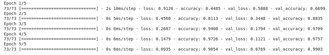
The output shows that our model achieves validation accuracy of 99.03% after 5 epochs.
Let’s now see how to create the above neural network model using the Functional API. The script below imports the Model, and the Input and Dense layers from the Keras library.
from keras.models import Model

from keras.layers import Input

from keras.layers import Dense
Let’s print the shape of our training data.
print(X_train.shape)
Output:
(1166, 4)
As discussed earlier, with functional API, you need to specify the input shape even in case of a DNN. To do so, you need to pass the number of columns to the “shape” attribute of the Input layer. In case of 2 dimensional tabular data, you can pass the number of attributes using X_train.shape[1].
inp_layer = Input(shape = X_train.shape[1], )
Next, to add layers, you need to pass the name of the previous layer in parenthesis after the next layer, until you reach the final or output layer.
dense = Dense(16, activation = 'relu')(inp_layer)

dense1 = Dense(8, activation = 'relu')(dense)

out_layer = Dense(1, activation= "sigmoid")(dense1)
To train the Keras model using the functional API, you need to pass the input and output layers to the Model class as shown below.
model_func = Model(inp_layer, out_layer)

model_func.compile(optimizer="adam", loss="binary_crossentropy", metrics=["accuracy"])
You can view your Keras model with the following script.
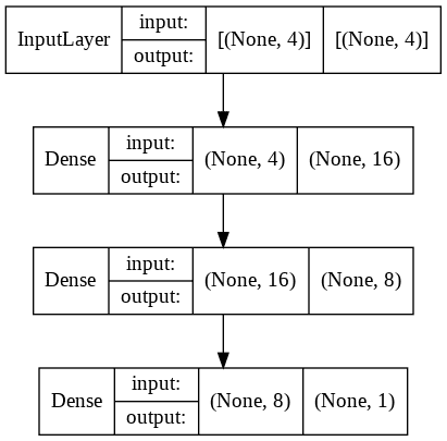
from keras.utils.vis_utils import plot_model

plot_model(model_func, to_file='model_plot.png', show_shapes=True, show_layer_names=False)
From the script below, you can see that the shape of our input is 4. Here None refers to the number of samples which can be any number depending upon the instances in your dataset.
Output:
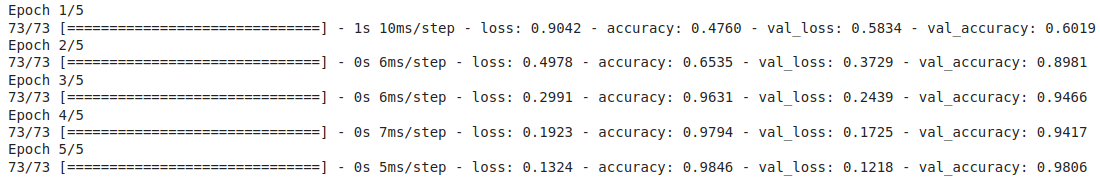
Finally the script below trains and validates our neural network model.
history = model_func.fit(X_train,

y_train,

epochs=5,

batch_size=16,

validation_data=(X_test, y_test))
Output:
Let’s now see how to create the above neural network model using the Functional API. The script below imports the Model, and the Input and Dense layers from the Keras library.
from keras.models import Model

from keras.layers import Input

from keras.layers import Dense
Let’s print the shape of our training data.
print(X_train.shape)
Output:
(1166, 4)
As discussed earlier, with functional API, you need to specify the input shape even in case of a DNN. To do so, you need to pass the number of columns to the “shape” attribute of the Input layer. In case of 2 dimensional tabular data, you can pass the number of attributes using X_train.shape[1].
inp_layer = Input(shape = X_train.shape[1], )
Next, to add layers, you need to pass the name of the previous layer in parenthesis after the next layer, until you reach the final or output layer.
dense = Dense(16, activation = 'relu')(inp_layer)

dense1 = Dense(8, activation = 'relu')(dense)

out_layer = Dense(1, activation= "sigmoid")(dense1)
To train the Keras model using the functional API, you need to pass the input and output layers to the Model class as shown below.
model_func = Model(inp_layer, out_layer)

model_func.compile(optimizer="adam", loss="binary_crossentropy", metrics=["accuracy"])
You can view your Keras model with the following script.
from keras.utils.vis_utils import plot_model

plot_model(model_func, to_file='model_plot.png', show_shapes=True, show_layer_names=False)
From the script below, you can see that the shape of our input is 4. Here None refers to the number of samples which can be any number depending upon the instances in your dataset.
Output:
Finally the script below trains and validates our neural network model.
history = model_func.fit(X_train,

y_train,

epochs=5,

batch_size=16,

validation_data=(X_test, y_test))
Output:
Image data type is another extremely important data type and is used to solve a variety of problems. The applications of algorithms trained via images are virtually endless. images are used to train driverless cars, to detect skin cancerous cells, to identify covid 19 using lung X-rays and so on.
TensorFlow Keras treats an image as a matrix with spatial relationships between different data points within a matrix. A grayscale image is treated as a single matrix. On other hand, a coloured image is treated as as a stacked combination of three matrices (one for each of the red, green, and blue colour channels)
- Unlike structured data, images have spatial relationships between different regions within an image. For example, in structured data like tables, swapping column locations had no effect on the dataset. On the other hand, swapping image regions affect the image dataset.
- Image datasets are difficult to manage owing to differences in shapes (height/width) and colour channels.
- Passing images directly to a DNN results in large dimensions of input data which can slow down model training. Further, a DNN is vulnerable to spatial variances between images. A convolutional neural network (CNN) is more suited to process image data.
As an example to understand the input shape for image data in Keras, you will be training a CNN model capable of classifying images in the fashion MNIST dataset. The fashion MNIST dataset contains images of various fashion items such as sneakers, pants, T-shirts, etc. The fashion MNIST dataset comes builtin with the Keras library.
The following script imports the required libraries for this section.
import numpy as np

import matplotlib.pyplot as plt

from tensorflow import keras

from keras.layers import Input, Conv2D, Dense, Flatten, Dropout, MaxPool2D

from keras.models import Model
The script below imports the fashion MNIST dataset and divides it into training and test sets.
mnist_images = keras.datasets.fashion_mnist

(X_train, y_train), (X_test, y_test) = mnist_images.load_data()
The images in the fashion MNIST dataset are greyscale where each pixel value is between 0 and 255. To normalise the dataset, the MNIST image pixels are divided by 255.0.
X_train, X_test = X_train/255.0, X_test/255.0
Let’s take a look at the shape of the training set.
print(X_train.shape)
Output:
(60000, 28, 28)
The result shows that there are 60 thousand images of 28 x 28 pixels in our training set.
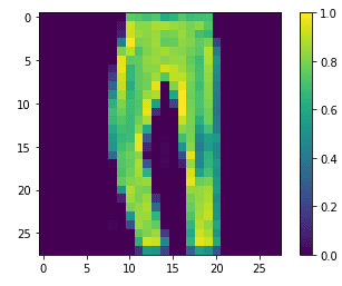
The following script plots the image and the 5th index in our test set.
#plotting image number 5 from test set
plt.figure()

plt.imshow(X_test[5])

plt.colorbar()

plt.grid(False)

plt.show()
Output:
You have seen earlier that the training and test set is currently in the form of (samples x height x width). However, a CNN in TensorFlow Keras expects input training images in the format (height x width x number of colour channels). Currently, we do not have a colour channel axis in our input images. The following script adds colour channel axes to the images in the training and test sets.
X_train = np.expand_dims(X_train, -1)

X_test = np.expand_dims(X_test, -1)

print(X_train.shape)

print(X_test.shape)
The output below shows that a colour channel has been added to the training and test images.
Output:
(60000, 28, 28, 1)
(10000, 28, 28, 1)
Let’s now see the shape of a single image because this is the shape that you will input to your CNN.
print(X_train[0].shape)
Output:
(28, 28, 1)
The following script prints the number of unique labels. This number will be used as the number of nodes in the output dense layer.
outputs = set(y_train)

print(outputs)
Output:
{0, 1, 2, 3, 4, 5, 6, 7, 8, 9}
Finally, the script below defines our Model. The model consists of two CNN layers ( a max pool layer which follows the first CNN layer), followed by a flatten layer, two dense layers, and finally an output dense layer.
inp_layer = Input(shape = X_train[0].shape )

conv1 = Conv2D(32, (3,3), strides = 2, activation= 'relu')(inp_layer)

maxp1 = MaxPool2D(2, 2)(conv1)

conv2 = Conv2D(64, (3,3), strides = 2, activation= 'relu')(maxp1)

flat1 = Flatten()(conv2)

dense1 = Dense(256, activation = 'relu')(flat1)

dense2 = Dense(128, activation = 'relu')(dense1)

out_layer = Dense(len(outputs), activation= 'softmax')(dense2)
The script below defines the model.
model_func = Model(inp_layer, out_layer)

model_func.compile(optimizer = 'adam', loss= 'sparse_categorical_crossentropy', metrics =['accuracy'])

And the script below displays  the model architecture.

from keras.utils.vis_utils import plot_model

plot_model(model_func, to_file='model_plot.png', show_shapes=True, show_layer_names=False)
Output:
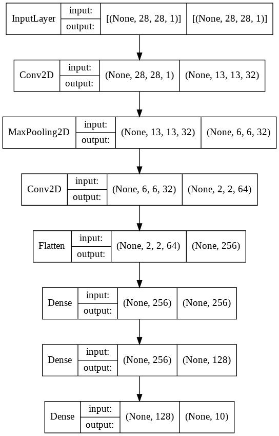
You can see from the above output that the shape of the input layer is 28 x 28 x 1 (Height x Width x Number of Colour Channels).
The rest of the process is familiar. The script below trains the model and prints the model accuracy on training and test set.
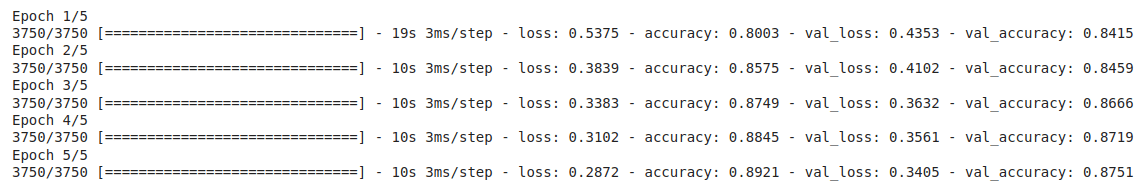
history = model_func.fit(X_train,

y_train,

epochs=5,

batch_size=16,

validation_data=(X_test, y_test))
Output:
The third important type of data that you will often come across while training your deep learning models is the sequence or time series data. Sequence data or the time series data is a type of data where the sequence in which the instances are recorded does matter. For instance, in case of stock market data, the stock prices on the day D are related and dependent on the stock prices on days D-1, D-2, and so on.
Similarly, text data is also a type of sequence data where the proceeding words depend upon the previously written words in a sentence.
- Sequence data is also a type of unstructured data where swapping instances can actually affect a model’s training performance. For instance, you cannot swap words occurring later in a sentence with the words occurring at the beginning, as it can totally change the semantic of a sentence.
- A DNN is not suited for training sequence data since a DNN treats all the time steps in the sequence data in parallel which kills the context information captured by the sequence. The Long Short Term Memory (LSTM) network, which is a type of a recurrent neural network, is more suited for processing sequence data.
In this section, you will see how to model a sequence problem for predicting an integer value using the LSTM model in TensorFlow Keras.
You will create your own dummy data for this section.
The script below imports the required libraries.
import numpy as np

import matplotlib.pyplot as plt

from tensorflow import keras

from keras.layers import Input, LSTM,  Dense

from keras.models import Model
The dummy dataset will consist of 15 instances (or samples) of 4 time steps each where each time step will consist of 2 features. To create such a dummy dataset, let’s define two lists that will correspond to 2 features in our dataset.
The first list consists of all the multiples of 6 upto 360, which results in 60 values. The second list consists of all the multiples of 3 up to 180 which also returns 60 values.
The script below creates the two feature lists:
f1 = np.array(range(6, 361, 6))

f2 = np.array(range(3, 181, 3))
The script below stacks the two feature lists horizontally and then prints the last 12 items as an example:
X = np.column_stack((f1, f2))

print(X[-12:])
Output:
[[294 147]
[300 150]
[306 153]
[312 156]
[318 159]
[324 162]
[330 165]
[336 168]
[342 171]
[348 174]
[354 177]
[360 180]]
The following script prints the shape of our feature set.
print(X.shape)
Output:
(60, 2)
Our feature set consists of 60 samples and two features. However, we want the feature set to be of the form 15 x 4 x 2 (15 samples, 4 time steps, 2 features per time step).
Run the script below to change the shape of the dataset. The script also prints the last 3 items from the dataset after changing the dataset shape.
X = np.array(X).reshape(15, 4, 2)

print(X[-3:])
Output:
[[[294 147]
[300 150]
[306 153]
[312 156]]
[[318 159]
[324 162]
[330 165]
[336 168]]
[[342 171]
[348 174]
[354 177]
[360 180]]]
Now if you look at the above output, you can see that the dataset consists of 4 time steps per sample, and two features per time step. Though the output only shows the last three samples (sample number 13, 14, and 15) for the sake of space, the total number of data samples is 15.
Let’s create a dummy output now. We want that for each input sample, the output is the sum of the two features in the last time step of every sample. For example, the two features in the 4th time step of the 15 samples are 360 and 180. The corresponding output will be 360 + 180 = 540.
y = [sum(x[-1]) for x in X]

y = np.array(y)

print(y)
Output:
[ 36 72 108 144 180 216 252 288 324 360 396 432 468 504 540]
Now we are ready to create our Model.
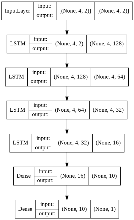
The LSTM, which is more suited to processing sequence data, accepts the input data in the format Time Steps, Features per time steps, which in our case is 4, 2, as you can see from the input layer in the script below.
Next, we add 4 LSTM layers and a dense layer, followed by the output dense layer.
inp_layer = Input(shape = (4,2))

lstm1 = LSTM(128, activation = "relu", return_sequences = True)(inp_layer)

lstm2 = LSTM(64, activation = "relu", return_sequences = True)(lstm1)

lstm3 = LSTM(32, activation = "relu", return_sequences = True)(lstm2)

lstm4 = LSTM(16, activation = "relu")(lstm3)

dense1 = Dense(10, activation = "relu")(lstm4)

out_layer = Dense(1)(dense1)
The rest of the process is familiar.
The following script compiles the model.
model_func = Model(inp_layer, out_layer)

model_func.compile(optimizer = "adam", loss= "mse")
The script below displays the model architecture.
from keras.utils.vis_utils import plot_model

plot_model(model_func, to_file='model_plot.png', show_shapes=True, show_layer_names=False)
Output:
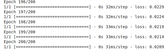
Finally, the script below trains the model.
history = model_func.fit(X,y, epochs = 200, verbose = 1)
Output:
To test our model, let’s predict the output value for a dummy instance. The dummy instance also consists of 4 time steps and 2 features. The output should be 390 + 195, since these are the feature values for the last time step.
test_data = np.array([[372, 186],

[378,189],

[384,192],

[390, 195]])

test_data = test_data.reshape((1, 4, 2))

output = model_func.predict(test_data, verbose=0)

print(output)
Output:
[[585.74396]]
In this article you briefly studied how to specify the input shapes for three main data types i.e. tabular data, images, and sequence data, when using these data types for training deep learning models developed in TensorFlow Keras library.
To summarise:
- For structured data, you can use the Keras sequential API where you do not need to specify the input data type. In the case of the Keras Functional API, you need to pass the (number of columns in your input table, ) to the shape attribute of the Input layer of the Keras library.
- For image data, the input should be specified in the form of (height, wight, number of colour channels)
- Finally, for sequence data, you need to pass a tuple (the number of time steps, features per time step) to the shape attribute of the Input layer of the Keras library.